代发新闻稿的网站毕业设计博客网站开发
文章目录
- 继承的基本使用
- 代码逐行讲解说明:
- 进阶案例
继承的基本使用
在现实生活中,继承一般指的是子女继承父辈的财产,父辈有的财产,子女能够直接使用。
程序里的继承
继承是面向对象软件设计中的一个概念,与多态、封装共为面向对象的三个基本特征。继承可以使得子类具有父类的属性和方法或者重新定义、追加属性和方法等。
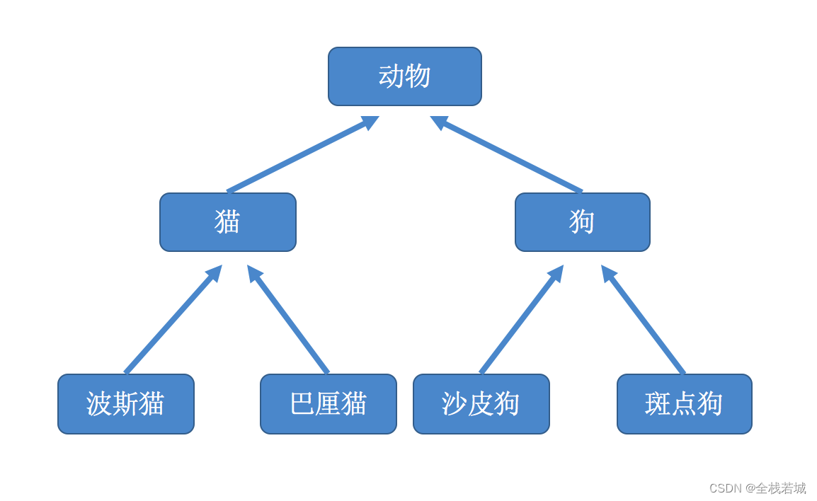
- 在程序中,继承描述的是多个类之间的所属关系。
- 如果一个类A里面的属性和方法可以复用,则可以通过继承的方式,传递到类B里。
- 那么类A就是基类,也叫做父类;类B就是派生类,也叫做子类。
class Animal:def __int__(self):pass"""动物类"""def sleep(self):print('正在睡觉')class Dog(Animal):"""Dog类继承自Animal类"""def __init__(self):passclass Cat(Animal): """Cat类继承自Animal类"""def __int__(self):pass# Dog 和 Cat 都继承自Animal类,可以直接使用Animal类里的sleep方法
dog = Dog()
dog.sleep()cat = Cat()
cat.sleep()
- 定义了一个基类
Animal,其中包含了一个方法sleep,用于输出动物正在睡觉。 Dog类和Cat类都继承自基类Animal,通过在类定义时将父类的类名放在括号内实现继承。- 实例化
Dog类和Cat类的对象分别为dog和cat。 - 调用
dog.sleep()和cat.sleep()方法,因为这两个方法来自于父类Animal,所以子类也能直接使用这些方法。 - 运行结果会依次输出 “正在睡觉”,表示
dog和cat都在睡觉。
代码逐行讲解说明:
class Animal:def __int__(self):pass"""动物类"""def sleep(self):print('正在睡觉')
- 定义了一个名为
Animal的基类,内部包含一个sleep方法,用于输出动物正在睡觉。
class Dog(Animal):"""Dog类继承自Animal类"""def __init__(self):pass
- 定义了一个名为
Dog的派生类,继承自基类Animal。通过将父类的类名放在括号内,实现了继承关系。
class Cat(Animal): """Cat类继承自Animal类"""def __int__(self):pass
- 定义了一个名为
Cat的派生类,同样继承自基类Animal。
# Dog 和 Cat 都继承自Animal类,可以直接使用Animal类里的sleep方法
dog = Dog()
dog.sleep()cat = Cat()
cat.sleep()
- 创建了一个
Dog类的对象dog并调用其sleep()方法,由于Dog类继承自Animal类,因此可以直接使用Animal类中定义的sleep()方法。 - 创建了一个
Cat类的对象cat并调用其sleep()方法,同样可以直接复用Animal类中的sleep()方法。
进阶案例
【Python】Python 实现猜单词游戏——挑战你的智力和运气!
【python】Python tkinter库实现重量单位转换器的GUI程序
【python】使用Selenium获取(2023博客之星)的参赛文章
【python】使用Selenium和Chrome WebDriver来获取 【腾讯云 Cloud Studio 实战训练营】中的文章信息
使用腾讯云 Cloud studio 实现调度百度AI实现文字识别
【玩转Python系列【小白必看】Python多线程爬虫:下载表情包网站的图片
【玩转Python系列】【小白必看】使用Python爬取双色球历史数据并可视化分析
【玩转python系列】【小白必看】使用Python爬虫技术获取代理IP并保存到文件中
【小白必看】Python图片合成示例之使用PIL库实现多张图片按行列合成
【小白必看】Python爬虫实战之批量下载女神图片并保存到本地
【小白必看】Python词云生成器详细解析及代码实现
【小白必看】Python爬取NBA球员数据示例
【小白必看】使用Python爬取喜马拉雅音频并保存的示例代码
【小白必看】使用Python批量下载英雄联盟皮肤图片的技术实现
【小白必看】Python爬虫数据处理与可视化
【小白必看】轻松获取王者荣耀英雄皮肤图片的Python爬虫程序
【小白必看】利用Python生成个性化名单Word文档
【小白必看】Python爬虫实战:获取阴阳师网站图片并自动保存
小白必看系列之图书管理系统-登录和注册功能示例代码
小白实战100案例: 完整简单的双色球彩票中奖判断程序,适合小白入门
使用 geopandas 和 shapely(.shp) 进行地理空间数据处理和可视化
使用selenium爬取猫眼电影榜单数据
图像增强算法Retinex原理与实现详解
爬虫入门指南(8): 编写天气数据爬虫程序,实现可视化分析
爬虫入门指南(7):使用Selenium和BeautifulSoup爬取豆瓣电影Top250实例讲解【爬虫小白必看】
爬虫入门指南(6):反爬虫与高级技巧:IP代理、User-Agent伪装、Cookie绕过登录验证及验证码识别工具
爬虫入门指南(5): 分布式爬虫与并发控制 【提高爬取效率与请求合理性控制的实现方法】
爬虫入门指南(4): 使用Selenium和API爬取动态网页的最佳方法
爬虫入门指南(3):Python网络请求及常见反爬虫策略应对方法
爬虫入门指南(2):如何使用正则表达式进行数据提取和处理
爬虫入门指南(1):学习爬虫的基础知识和技巧
深度学习模型在图像识别中的应用:CIFAR-10数据集实践与准确率分析
Python面向对象编程基础知识和示例代码
MySQL 数据库操作指南:学习如何使用 Python 进行增删改查操作
Python文件操作指南:编码、读取、写入和异常处理
使用Python和Selenium自动化爬取 #【端午特别征文】 探索技术极致,未来因你出“粽” # 的投稿文章
Python多线程与多进程教程:全面解析、代码案例与优化技巧
Selenium自动化工具集 - 完整指南和使用教程
Python网络爬虫基础进阶到实战教程
Python入门教程:掌握for循环、while循环、字符串操作、文件读写与异常处理等基础知识
Pandas数据处理与分析教程:从基础到实战
Python 中常用的数据类型及相关操作详解
【2023年最新】提高分类模型指标的六大方案详解
Python编程入门基础及高级技能、Web开发、数据分析和机器学习与人工智能
用4种回归方法绘制预测结果图表:向量回归、随机森林回归、线性回归、K-最近邻回归